We presente a Generative Adversarial Network designed to perform audio inpainting on magnitude spectrums. This architecture can be deployed int two ways denoted CIGAN and PIGAN CIGAN reconstructs the magnitude spectrum of an audio frame of length T seconds, given the previous and subsequent T seconds. PIGAN, instead, is more similar to the concept perform audio prediction. It can be trained to predict an audio frame of T seconds, given the T previous seconds. This web page accompains the github repository.
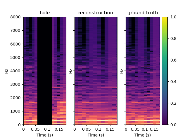
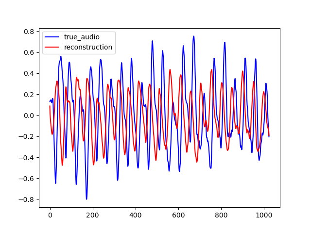
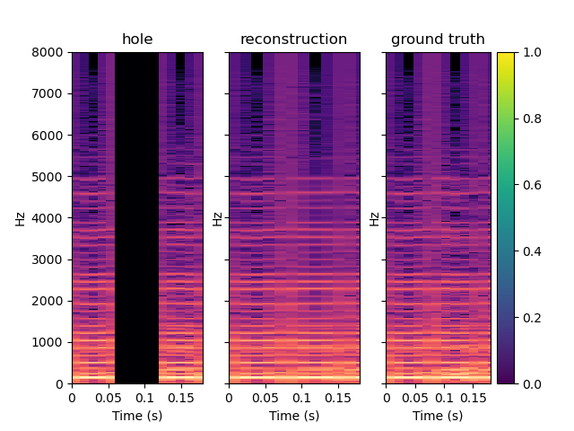
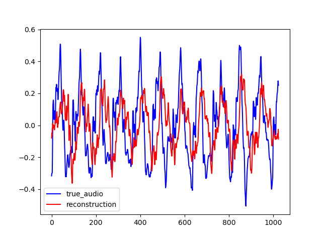
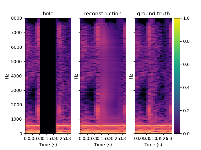
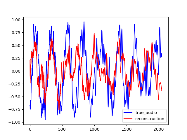
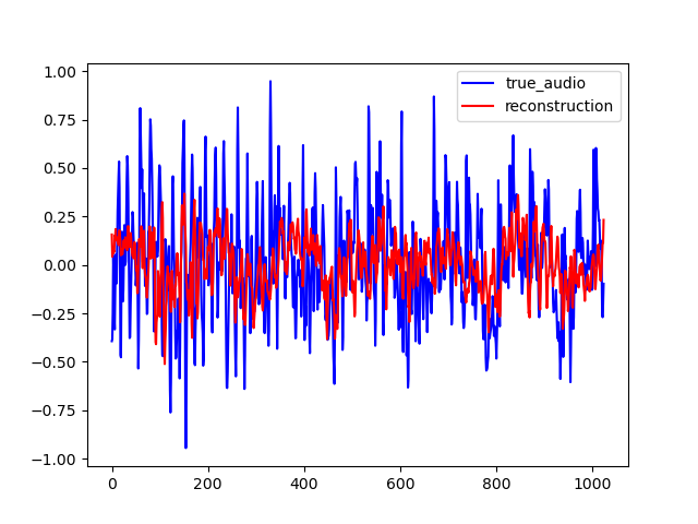
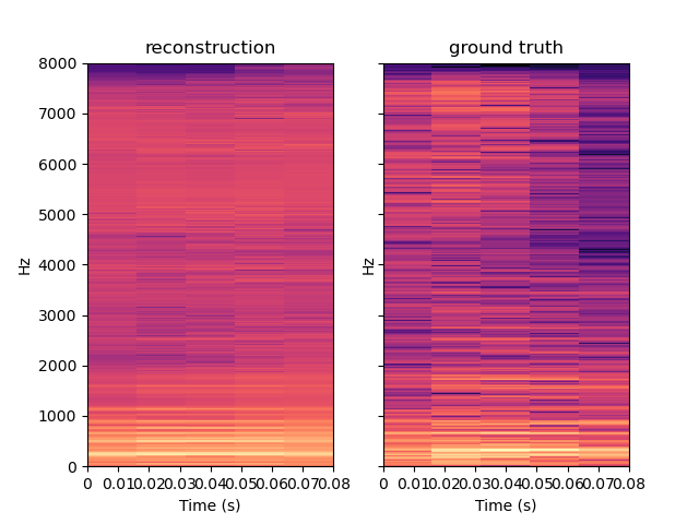
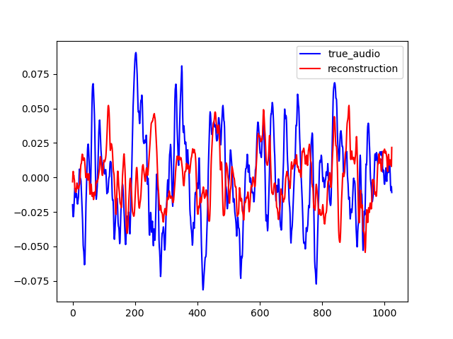
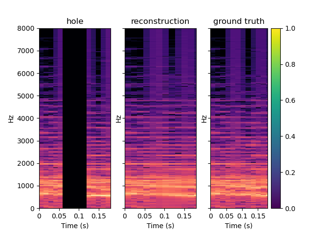
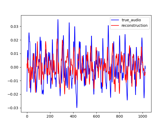
Here are some samples output by CIGAN for T=0.064. To reconstruct the audio from the magnitude spectrums, the Griffin-Lim algorithm was used. As shown in the various examples, the reconstructed spectrums are rather good, even if they are blurred. The audio waveforms look similar to the ground truth even if they are not close from them. It might be because the Griffin-Lim does not output the exact waveform, even if it is fed with the real magnitude. Moreover, it works from an approximation of the real magnitude spectrum. To obtain this result, CIGAN was trained for 200 epochs on the small FMA dataset.
| Spectrum | Waveform |
|---|---|
|
|
|
|
|
|
|
|
| Original Audio | Reconstructed Audio |
|---|---|
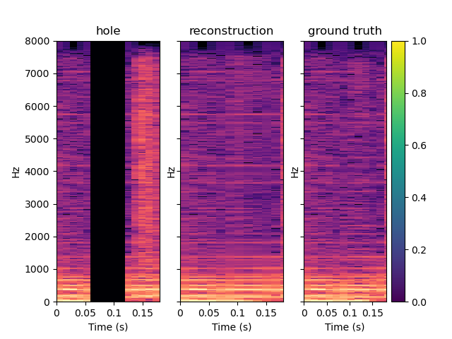
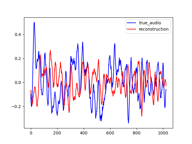
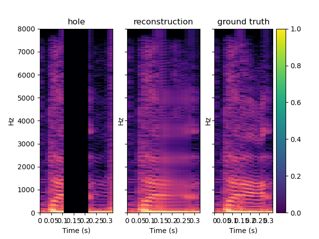
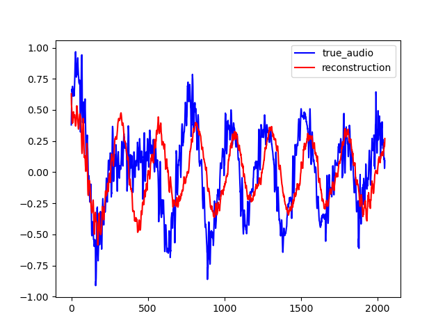
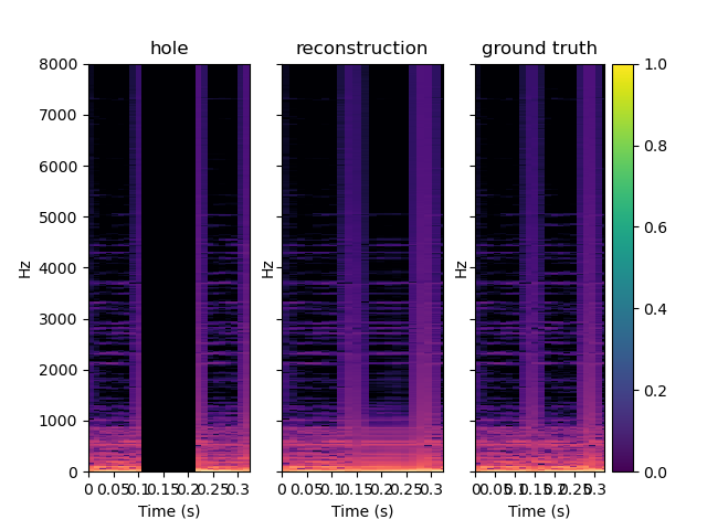
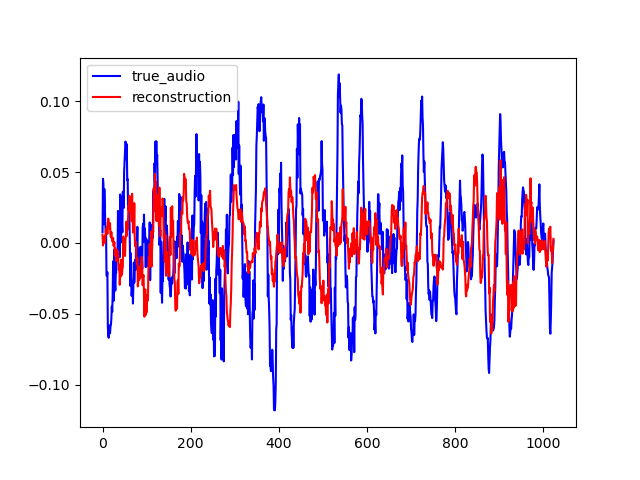
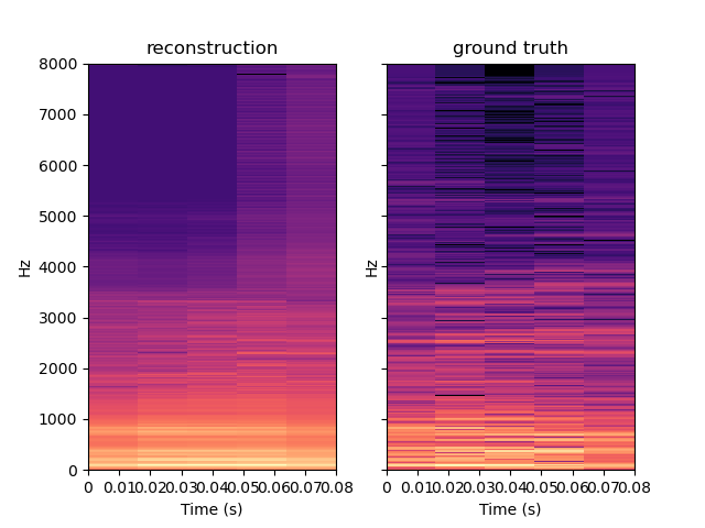
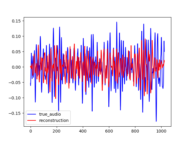
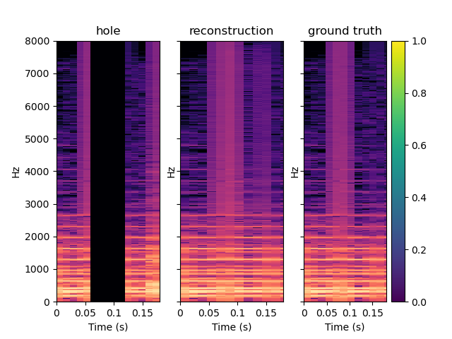
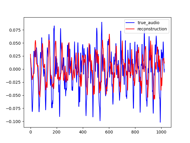
Here are other samples for T=0.128 s. One can notice that the reconstruction quality is lower, especially in the first example which is a bad one.
| Spectrum | Waveform |
|---|---|
 |
|
| 
|
|
|
| Original Audio | Reconstructed Audio |
|---|---|
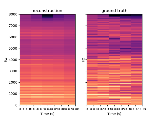
PIGAN is an adaptation of the network in order to achieve audio prediction. The neural network predicts the magnitude spectrum of an audio frame of length T given the T previous seconds. On the examples below, one can see that PIGAN perform less well than CIGAN. It is because the new task is much more challenging. However, the result are still interesting. The example are obtained with T = 0.064 s.
| Spectrum | Waveform |
|---|---|
 |
|
| 
|
| 
|
| Original Audio | Reconstructed Audio |
|---|---|
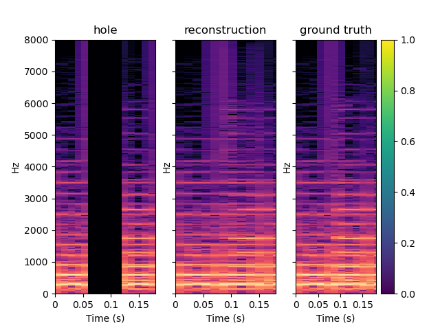
To perceptually evaluate the model, we use it to fill in one gap of T = 0.064 s, located at 0.5 s in an audio sample of two seconds. Then, we run a matlab function to compute the ODG between the original audio and the audio with the filled gap. The examples below are obtained with CIGAN with T = 0.064 s.
On the last example of this section, one can heard that CIGAN does its job. Indeed, it is very difficult to heard a difference between the original and the reconstructed one while the difference is audible between the original audio and the one with the hole. In the second example, it is difficult to heard a difference between the original audio, and the one with the hole. This is probably because the hole come when the song is rather silent. Still, we can notice that IGAN doesn't put annoying noise instead of the silence.
| Original Audio | Reconstructed Audio | Audio with hole |
|---|---|---|
The considered frame length, 0.064 s, is very short. Previously, we fill in a gap 0.064 ms in an audio of 2s length. In this experiment, we reconstruct the whole 2s long audio by frame of 64ms. Each frame of 64 ms are reconstructed using CIGAN, with as input the previous and subsequent 64 ms, taken from the original audio. Then, all the predicted frames are concatenated together. As shown in the examples below, the audios are easily recognizable, even if they are noisy. The noise might come from a possible discontinuity at the intersection of two frames.
| Original Audio | Reconstructed Audio |
|---|---|
In this experiment, we do the same than previously, but with PIGAN. Each frame of 64ms are first reconstructed using PIGAN, with as input the previous frame, taken from the original audio. Then, all the predicted frames are concatenated together. As shown in the examples below, the audios are easily recognizable, even if they are noisy.
| Original Audio | Reconstructed Audio |
|---|---|
To test our model generalization ability, we used it to inpaint on the MAESTRO dataset while training it on the small version of the FMA dataset. The FMA dataset is composed of 3000 tracks of 30s of 8 different music styles while the MAESTRO dataset is composed of classical piano records. The example below are obtained with CIGAN with T = 0.064. When comparing these examples with the ones shown previously, one can see that CIGAN behaves in the same way in both case. Thus, the model generalization ability seems to be nice.
| Spectrum | Waveform |
|---|---|
|
|
| 
|
| 
|
| Original Audio | Reconstructed Audio |
|---|---|
"Enabling Factorized Piano Music Modeling and Generation with the MAESTRO Dataset." , Curtis Hawthorne, Andriy Stasyuk, Adam Roberts, Ian Simon, Cheng-Zhi Anna Huang, Sander Dieleman, Erich Elsen, Jesse Engel, and Douglas Eck. In International Conference on Learning Representations, 2019.
A Dataset for Music Analysis, Defferrard, Michael and Benzi, Kirell and Vandergheynst, Pierre and Bresson, Xavier. In 18th International Society for Music Information Retrieval Conference (ISMIR)